|
trantute2 (OP)
|
 |
August 17, 2018, 07:12:25 PM
Last edit: August 17, 2018, 07:31:04 PM by trantute2 |
|
Es geht um B. Der Dreiecks-Tausch findet auf einer Börse statt, weil es sonst zu langsam wäre. Orderbücher müsst ich erst konstruieren, damit der Tausch mit den Beispiel Daten auch Gewinn macht.
Das macht die ganze Geschichte etwas einfacher. Das Beispiel, welches ich oben gegeben habe ist ein Spezialfall, wo man auf einer Börse handelt und das Orderbuch nur einen Preis mit unbegrenztem Volumen enthält. Die Idee ist jetzt, dass man die eine Variable für ein Tauschpaar aufsplittet sodass es Variablen für jeden Preiseintrag im Tauschpaar-Orderbuch gibt. Z.B. bei einem Orderbuch mit 1 BTC bei $6000, 1.5 BTC bei $6100 und 0.5 BTC bei $6200 bräuchte man drei Variablen. Die Anzahl der Variablen hängt also von der Feinkörnigkeit des Orderbuchs ab. Aus jeder Spalte im LP-Arbitragebeispiel wird dann eine ganze Matrix. Der Aufwand bleibt aber trotzdem überschaubar, da auch die Orderbücher überschaubar sind. LP-Probleminstanzen sind hauptsächlich durch den Speicher begrenzt, aber selbst Grössen jenseits mehrerer 100 MB sollten kein Problem sein. Ich tippe hier aber eher auf kB, wenn es hoch kommt sind das ein paar MB. Das Volumen, welches pro Preis vorhanden und als "Fluss" maximal "fliessen" kann, sollte als zusätzliche, ziemlich simple Bedingungen analog den "x1 <= 10000" machbar sein. Ganz sicher bin ich mir natürlich nicht ob das funktioniert. Ich würde/werde mir einfach ein kleines Toyexample basteln und ein bisschen rumspielen. Interessant ist das Problem allemal. Eben weil es eine praktische Anwendung ist. Die Ergebnisse können wir ja dann vergleichen, Deine Methode vs. meine um zu gucken ob die jeweilige Lösung macht was sie soll. Hab im Moment leider sehr wenig Zeit...  Geht mir genauso, deswegen kann ich Dir keine Garantie geben, ob und wann ich eine entsprechende LP-Formulierung zusammenfrickeln kann. Falls nicht, dann muss beschriebene Idee ausreichen (falls sie denn überhaupt funktioniert). |
|
|
|
|
|
|
|
|
|
|
|
|
|
There are several different types of Bitcoin clients. The most secure are full nodes like Bitcoin Core, but full nodes are more resource-heavy, and they must do a lengthy initial syncing process. As a result, lightweight clients with somewhat less security are commonly used.
|
|
|
Advertised sites are not endorsed by the Bitcoin Forum. They may be unsafe, untrustworthy, or illegal in your jurisdiction.
|
|
|
|
|
|
|
|
arunka71
|
|
August 17, 2018, 08:41:02 PM |
|
Ehrlich gesagt sollte man aus meiner Sicht gerade nicht soviel Zeit in dieses Problem investieren, weil dieses Konzept im Moment (zumindest mit meinen Mitteln) nicht wirklich funktioniert. Dieser Bot ist von 2012, und da gab es eine Zeit wo das mal recht gut ging.
Angeblich hat es vor einer Weile wieder funktioniert, aber dafür muss man dann echt fixen Code haben. Da sind die Rechnungen, die man dann noch machen kann eher beschränkt. Weiss nicht, ob man dann noch mit grossen Matrizen rumrechnen sollte.
|
|
|
|
|
|
trantute2 (OP)
|
|
August 18, 2018, 09:32:21 AM |
|
Ehrlich gesagt sollte man aus meiner Sicht gerade nicht soviel Zeit in dieses Problem investieren, weil dieses Konzept im Moment (zumindest mit meinen Mitteln) nicht wirklich funktioniert. Dieser Bot ist von 2012, und da gab es eine Zeit wo das mal recht gut ging.
Angeblich hat es vor einer Weile wieder funktioniert, aber dafür muss man dann echt fixen Code haben. Da sind die Rechnungen, die man dann noch machen kann eher beschränkt. Weiss nicht, ob man dann noch mit grossen Matrizen rumrechnen sollte.
Wenn Du sagst, dass Dein Code zu langsam wäre/war: Über welche Zeiträume reden wir denn hier? Sekunden, Millisekunden oder gar Mikrosekunden? Das LP selbst ist schnell erzeugt und besteht nur aus einem String. Die limitierenden Faktoren sind, diesen String als Datei zu schreiben, vom Solver einlesen zu lassen, die Lösung vom Solver schreiben zu lassen und diese wieder einzulesen und zu analysieren. Die Zeit für das Lösen des Problem ist imho vernachlässigbar, denn die Solver für LPs sind verdammt schnell. |
|
|
|
|
|
arunka71
|
|
August 18, 2018, 09:53:00 PM |
|
Kommt drauf an. Der damalige Bot war sehr lahm und damals hätten sicherlich Millisekunden gereicht. Aber das funktioniert ja wohl nicht mehr, weshalb man heute schnellere Verbindungen braucht, und sich das eher in den Mikrosekunden Bereich verschieben wird, wenn man stabil Erfolg haben will.
|
|
|
|
|
|
trantute2 (OP)
|
|
August 19, 2018, 09:22:01 AM |
|
Wahrscheinlich versuchen einige computergestützte Arbitrage direkt auf der selben Börse und dadurch wird die Anzahl der Arbitragemöglichkeiten minimiert ...
|
|
|
|
|
|
arunka71
|
|
August 19, 2018, 09:36:16 PM |
|
Joar. Zu der Zeit, als btc-e das noch angezeigt hat, waren ja manchmal > 1000 Bots unterwegs. Da entscheidet dann halt der schnellste Zugriff...
|
|
|
|
|
|
trantute2 (OP)
|
|
November 04, 2018, 08:19:24 PM |
|
Was Neuronale Netze angeht und damit möglicherweise eine Methode den Kurs direkt vorherzusagen: https://machinelearningmastery.com/multi-step-time-series-forecasting-long-short-term-memory-networks-python/Man kann z.B. die Bitstamp-Daten aus dem HMM-Teil dazu nehmen. Ich habe das mal testweise ausprobiert. Das sieht aber noch nicht so toll aus. Ausserdem vestehe ich den Grossteil der Methode noch nicht. Nichtmal ansatzweise! Neuronale Netze sind ein PITA, JFR. D.h. eine genauere Analyse fehlt noch, ich arbeite dran ... (Einfach mal, um auch diesen Thread wieder hochzuholen  ) |
|
|
|
|
|
trantute2 (OP)
|
|
November 13, 2018, 06:31:07 PM |
|
Teaser:  Oberes ist eine Bitcoin-Return-Vorhersage für Samstag, den 16.11.2018 (US-Zeit). Für "Return" siehe auch https://bitcointalk.org/index.php?topic=4586924.0#post_drei. Die x-Achse stellt die vergangene Zeit in Wochen dar, die y-Achse den Return, welcher dimensionlos ist. D.h, ist der Wert des violetten Knubbels negativ, dann fällt der Kurs bis zum US-Börsenschluss (SP500) am jeweils kommenden Freitag relativ zum Freitag davor. Wenn der Return steigt, dann ist der violette Knubbel im positiven Bereich. Dabei ist der blaue Plot der historische Return, der violette Plot ist das gelernten Modell ohne den Error-Term (mit Error-Term wäre dies exakt der blaue Plot, "Error" steht hierbei für "unbekannter Einfluss auf Daten") und der violette Knubbel ist die Vorhersage für den kommenden Freitag. Unten auf der x-Achse sieht man ein rot-grünes Band, welches anzeigt, wann das gelernte Model ohne Error-Term auf der richtigen Seite lag (rot = falsch, grün = richtig), d.h. wo befindet sich die blaue Linie relativ zur Null und wo die Violette. Wohlgemerkt ist das Modell wahrscheinlich overfittet. Crossvalidierung etc. pp. habe ich (noch) nicht durchgeführt. Ich stelle den mal hier rein um zu gucken, ob wir am Ende wirklich Minus machen. Im Nachhinein den Plot zu posten, wenn man schon weiss, wie sich er Kurs bewegt, das wäre schlicht zu lame. Ich habe vier Methoden rumliegen, welche sich am gleichen, aber erweiterbaren Datensatz orientieren. Diese sind eng miteinander verwandt, also erwartet keine Wunder. Ich möchte aber, auch für mich selbst, einfach mal vergleichen, ob es da Unterschiede in der Vorhersagekraft gibt. Nichtsdetotrotz sind die Parameter noch lange nicht optimal gewählt, d.h. es könnte noch viel Luft nach oben geben. Code etc. pp.: folgt irgendwann Quellen: keine |
|
|
|
|
|
cypher21
|
|
November 13, 2018, 06:45:56 PM |
|
finde sehr gut das du ein wenig herum tüftelst und uns deine Ergebnisse auch mitteilst. Mach weiter so  Ich verfolge das auf jeden Fall mit Interesse. Merit dafür |
|
|
|
|
|
trantute2 (OP)
|
|
December 10, 2018, 06:09:56 AM |
|
Das Bashskript für den Faktorendownload: #!/bin/bash
rm *.csv
rm *.tar.gz
wget https://coinmetrics.io/data/all.tar.gz
tar -xzvf all.tar.gz
Am besten kommt das in einen Ordner mit Namen "coinmetrics" rein, dann klappt auch das folgende R-Skript, welches sich direkt ausserhalb des Ordners befindet. Der Code ist super hässlich, enthält redundante Sachen oder Kram, welcher vom Debugging stammt und lässt sich bestimmt noch optimieren. Auch die Variablennamen sind teils nichtssagend. Ich hoffe, den demnächst überarbeiten zu können: keep_cols <- function(data, keep=NULL){
if (is.null(keep))
return(data);
to_keep <- rep(FALSE, ncol(data));
for (k in keep)
to_keep <- to_keep | grepl(k, colnames(data));
ret <- data[,to_keep];
ret <- ret[,order(colnames(ret))];
return(ret);
}
merge_data <- function(data, keep=NULL, drop_cols=FALSE){
ret <- NULL;
for (i in 1:length(data)){
if (is.null(keep) || names(data)[i] %in% keep){
datum <- data[[i]];
if (drop_cols)
datum <- datum[,!is.na(datum[nrow(datum),])]
index <- which(grepl("date", colnames(datum)));
if (length(index) == 1){
if (is.null(ret)){
ret <- datum;
byx <- colnames(datum)[index];
} else {
byy <- colnames(datum)[index];
ret <- merge(x=ret, y=datum, by.x=byx, by.y=byy);
}
}
}
}
return(ret);
}
read_dir <- function(dir){
files <- list.files(dir, pattern="*.csv");
ret <- list();
for (file in files){
datum <- read.csv(file=paste(dir, file, sep="/"));
colnames(datum) <- paste(file, colnames(datum), sep=".");
ret <- append(ret, list(datum));
}
names(ret) <- files;
return(ret);
}
make_open_close <- function(data, number_of_days=7, date="DATE", price="PRICE"){
x <- data;
# extrahiere ersten und letzten Tag der Woche
if (number_of_days > 1){
x <- cbind(x, "WEEK_DAY"=((1:nrow(x))%%number_of_days));
open <- x[x$WEEK_DAY==1, price];
close <- x[x$WEEK_DAY==0, price];
open_date <- x[x$WEEK_DAY==1, date];
close_date <- x[x$WEEK_DAY==0, date];
} else {
open <- x[,price];
close <- x[,price];
open_date <- x[,date];
close_date <- x[,date];
}
# passe die Länge der Vektoren an sodass es für jeden Tag eine Entsprechung gibt, einer der Fälle ist glaube ich unnötig
if (length(open) > length(close)) {open <- open[1:length(close)]; open_date <- open_date[1:length(close)];};
if (length(open) < length(close)) {close <- close[1:length(open)]; close_date <- close_date[1:length(open)];};
return(data.frame("OPEN_DATE"=open_date, "CLOSE_DATE"=close_date, "OPEN_PRICE"=open, "CLOSE_PRICE"=close));
}
make_return <- function(data){
return((data$CLOSE_PRICE - data$OPEN_PRICE)/data$OPEN_PRICE);
}
test_levels <- function(data, id=NULL){
if (!is.null(id))
print(id);
bar <- table(data);
print(bar[bar == 1]);
}
make_breaks <- function(data, breaks=5, ignore=c()){
ret <- data;
for (i in 3:ncol(ret))
if (!(colnames(ret)[i] %in% ignore))
ret[,i] <- cut(ret[,i], breaks=breaks);
return(ret);
}
make_formula <- function(data, y=NULL, ignore=c()){
if (is.null(y))
stop("id for y-variable missing");
ret <- paste(setdiff(colnames(data), c(y, ignore)), collapse=" + ");
ret <- paste(y, ret, sep=" ~ ");
return(ret);
}
make_prediction <- function(data, price_id=NULL, shift=1, breaks=5, ignore=c()){
if (is.null(price_id))
stop("price_id missing");
R <- make_breaks(data, breaks=breaks, ignore=price_id);
shifted_R <- R;
shifted_R[1:(length(R[,price_id])-shift), price_id] <- R[(shift+1):length(R[,price_id]), price_id];
shifted_R <- shifted_R[1:(length(R[,price_id])-shift),];
formula <- make_formula(shifted_R, y=price_id, ignore=ignore);
shifted_fit <- lm(formula, data=shifted_R);
to_predict <- R[(nrow(R)-shift+1):nrow(R),];
to_predict[,price_id] <- NA;
# were levels for prediction used in fit?
b <- rep(TRUE,3); for (i in 4:length(to_predict)){b <- c(b, to_predict[1,colnames(to_predict)[i]] %in% shifted_R[,colnames(to_predict)[i]])}
if (sum(!b) > 0)
cat(paste("New levels: ", paste(colnames(to_predict)[!b], collapse=", "), sep=""));
# replace non-existing factors with last one in shifted_R
# actually it should be better to use factor from fit, which is closest
to_predict[1,!b] <- shifted_R[nrow(shifted_R),!b];
prediction <- predict(shifted_fit, to_predict);
ret <- list(prediction, to_predict, R, shifted_R, shifted_fit);
names(ret) <- c("PREDICTION", "TO_PREDICT", "R", "SHIFTED_R", "SHIFTED_FIT");
return(ret);
}
breaks = 15;
price_id = "btc.csv.price.USD.";
x <- read_dir("coinmetrics");
x <- merge_data(x, keep=c("btc.csv", "ltc.csv", "eth.csv", "xrp.csv", "doge.csv", "usdt.csv", "gold.csv", "sp500.csv"), drop_cols=TRUE);
x <- keep_cols(x, c("btc.csv.date", "price", "value", ".txVolume.", "marketcap"));
colnames(x)[colnames(x)=="btc.csv.date"] <- "DATE";
# simply switches columns:
index <- which(colnames(x)==price_id);
indices <- 1:ncol(x);
indices[2] <- index;
indices[index] <- 2;
x <- x[,indices];
x <- x[apply(x, MARGIN=1, function(ret){!any(is.na(ret))}),];
x <- x[(nrow(x) %% 7 + 1):nrow(x),];
R <- make_open_close(x, price=price_id)[,c("OPEN_DATE", "CLOSE_DATE")];
for (i in 2:ncol(x))
R <- cbind(R, make_return(make_open_close(x, price=colnames(x)[i])));
colnames(R)[3:length(colnames(R))] <- colnames(x)[2:length(colnames(x))];
#R <- R[1:(nrow(R)-1),];
svd_R <- R;
foo <- make_prediction(R, price_id=price_id, shift=1, breaks=breaks, ignore=c("OPEN_DATE", "CLOSE_DATE"));
prediction <- foo$PREDICTION;
R <- foo$R;
shifted_R <- foo$SHIFTED_R
shifted_fit <- foo$SHIFTED_FIT;
# evaluations
X <- model.matrix(shifted_fit);
beta <- coefficients(shifted_fit);
X <- X[,!is.na(beta)];
beta <- beta[!is.na(beta)];
evaluation_historically <- X %*% beta;
correct_predictions <- (evaluation_historically < 0) == (shifted_R[,price_id] < 0);
print(sum(correct_predictions)/nrow(shifted_R));
n <- 10^8; print(sum((ceiling(runif(n)*nrow(shifted_R)) <= sum(shifted_R[,price_id] < 0)) == (ceiling(runif(n)*nrow(shifted_R)) <= sum(shifted_R[,price_id] < 0)))/n);
dev.new(width=19, height=3.5);
matplot(R[,price_id], type="l", col=c("blue"), lty = c(1), xaxt="n");
abline(h=0, col="black");
lines((1:length(evaluation_historically))+1, evaluation_historically, col="violet");
points(length(R[,price_id])+1, prediction, col="violet", pch=16);
ops <- c(0.06927308);
old_predictions <- data.frame("x"=(nrow(R)-length(ops)+1):nrow(R), "y"=ops);
points(old_predictions$x, old_predictions$y, col="violet", pch=1);
int <- floor(nrow(R)/7) - 1; # warum auch immer minus 1?
axis(1, at = int*(0:7)+1, labels = R$CLOSE_DATE[int*(0:7)+1]);
legend("left", legend = c("historic", "learned"), col = c("blue", "violet"), lty = c(1,1), lwd = 1 , xpd = T );
title(paste("Weekly BTC return prediction via factorial regression (breaks = ", breaks, "):\nPredicted return for ", as.Date(R$CLOSE_DATE[nrow(R)])+7, ": ", prediction, sep=""));
min_val <- min(c(R[,price_id], evaluation_historically));
colors <- c("red", "green");
correct_predictions <- (evaluation_historically < 0) == (shifted_R[,price_id] < 0);
correct_predictions <- as.integer(correct_predictions)+1;
for (i in 1:length(correct_predictions)){rect(i+1-0.5, min_val, i+2-0.5, min_val-0.1, col=colors[correct_predictions[i]], border=NA)}
factors <- tail(colnames(R),-3);
f1 <- paste(factors[1:14], collapse=", ");
f2 <- paste(factors[15:19], collapse=", ");
s <- paste(f1, f2, sep=",\n")
title(sub=s, adj=0, line=3, font=2, cex.sub=0.9);
|
|
|
|
|
|
|
|
|
|
trantute2 (OP)
|
|
June 08, 2020, 06:17:26 AM |
|
Habe den HMM auf python3 umgestellt, da - die HMM-Funktion in R nicht mehr konvergiert bzw. eine Fehlermeldung zurückgibt (warum auch immer),
- die Datenprozessierung schneller ist,
- es weniger Speicher braucht.
import os;
import wget;                # pip3 install wget
import numpy;               # pip3 install numpy
import pandas;              # pip3 install pandas
import matplotlib;          # pip3 install matplotlib
from hmmlearn import hmm;   # pip install --upgrade --user hmmlearn

######################################################################

# weighted mean
def wm(x):
    return (x['VOLUME'] * x['PRICE']).sum()/x['VOLUME'].sum();

# removes incomplete weeks
def rm(df, column, n):
    for i in range(n):
        if df[column].iloc[0] != subdata[column].iloc[i]:
            return df.iloc[i:df.shape[0]];
    return df;

def fill(df, column):
    x = numpy.zeros([df.shape[0]]);
    c = 0; x[0] = c;
    for i in range(df.shape[0]-1):
        if df[column].iloc[i] != df[column].iloc[i+1]:
            c += 1;
        x[i+1] = c;
    return x.astype(int);

######################################################################

# download and/or load bitstamp data
file_name = 'bitstampUSD.csv.gz';
# but make sure, that the file is up to date
if os.path.exists(file_name) == False:
    file_name = wget.download('https://api.bitcoincharts.com/v1/csv/bitstampUSD.csv.gz');

data = pandas.read_csv(file_name, compression='gzip', header=None);
data.columns = ['EPOCH', 'PRICE', 'VOLUME'];
data = data.sort_values(by='EPOCH');
data['DATE'] = pandas.to_datetime(data['EPOCH'],unit='s').dt.tz_localize('utc').dt.tz_convert('Europe/Berlin');
data['DAY'] = [str(x) for x in pandas.Series(data['DATE']).dt.date];

# firstly group by day for faster processing
subdata = data.groupby('DAY').first();
subdata['OPEN'] = data.groupby('DAY').first()['PRICE'];
subdata['CLOSE'] = data.groupby('DAY').last()['PRICE'];
subdata['MAX'] = data.groupby('DAY').max()['PRICE'];
subdata['MIN'] = data.groupby('DAY').min()['PRICE'];
subdata['VOLUME'] = data.groupby('DAY').sum()['VOLUME'];

subdata['PRICE'] = data.groupby(['DAY']).apply(wm);
subdata['MA50'] = subdata["MAX"].rolling(50).mean();
subdata['MA200'] = subdata["MAX"].rolling(200).mean();
subdata['RETURN'] = (subdata['CLOSE'] - subdata['OPEN'])/subdata['OPEN'];

subdata['WEEK'] = [str(pandas.Timestamp(x).week) for x in subdata['DATE']];

######################################################################
# not very elegant way to get unique week annotation

# remove first incomplete WEEK
subdata = rm(subdata, 'WEEK', 7);

# remove last incomplete WEEK
subdata = subdata.sort_values(by='EPOCH', ascending=False);
subdata = rm(subdata, 'WEEK', 7);
subdata = subdata.sort_values(by='EPOCH');

subdata['WEEK'] = fill(subdata,'WEEK');

######################################################################

# secondly group by week
subsubdata = subdata.groupby('WEEK').first();
subsubdata['DAY'] = [str(x) for x in pandas.Series(subsubdata['DATE']).dt.date];
subsubdata['OPEN'] = subdata.groupby('WEEK').first()['OPEN'];
subsubdata['CLOSE'] = subdata.groupby('WEEK').last()['CLOSE'];
subsubdata['MAX'] = subdata.groupby('WEEK').max()['MAX'];
subsubdata['MIN'] = subdata.groupby('WEEK').min()['MIN'];
subsubdata['VOLUME'] = subdata.groupby('WEEK').sum()['VOLUME'];
subsubdata['PRICE'] = subdata.groupby(['WEEK']).apply(wm);
subsubdata['LOG10_PRICE'] = numpy.log10(subsubdata['PRICE']);
subsubdata['LOG10_PRICE'] = subsubdata['LOG10_PRICE']/numpy.amax(subsubdata['LOG10_PRICE']);
subsubdata['LOG10_MA50'] = numpy.log10(subsubdata['MA50']);
subsubdata['LOG10_MA50'] = subsubdata['LOG10_MA50']/numpy.amax(subsubdata['LOG10_MA50']);
subsubdata['LOG10_MA200'] = numpy.log10(subsubdata['MA200']);
subsubdata['LOG10_MA200'] = subsubdata['LOG10_MA200']/numpy.amax(subsubdata['LOG10_MA200']);
subsubdata['RETURN'] = (subsubdata['CLOSE'] - subsubdata['OPEN'])/subsubdata['OPEN'];

# at least not wrong ...
subsubdata = subsubdata.sort_values(by='EPOCH');

# create a model and fit it to data
model = hmm.GaussianHMM(4, "diag", n_iter=1000);

X = numpy.asarray(subsubdata['RETURN']).reshape(-1,1);
fit = model.fit(X);

hidden_states = model.predict(X);
hidden_probs = model.predict_proba(X);
df = pandas.DataFrame(hidden_probs);
df.columns = ['0', '1', '2', '3'];

# my sentiment definition
bubble_state = hidden_states[numpy.where(subsubdata['DATE']=='2011-09-19 15:47:03+0200')[0][0]];
sideways_state = hidden_states[numpy.where(subsubdata['DATE']=='2016-10-03 00:00:18+0200')[0][0]];
bullish_state = hidden_states[numpy.where(subsubdata['DATE']=='2013-02-11 00:57:24+0100')[0][0]];
bearish_state = list(set([0,1,2,3]).difference([bubble_state, sideways_state, bullish_state]))[0];

state_index = {'violet':str(bubble_state), 'green':str(bullish_state), 'black':str(sideways_state), 'red':str(bearish_state)};
state_index_= {str(bubble_state):'violet', str(bullish_state):'green', str(sideways_state):'black', str(bearish_state):'red'};

# plot the result
import matplotlib.pyplot as plt;

fig, ax = plt.subplots(figsize=(2.24,2.24));
df[state_index['violet']].plot(ax=ax, color='violet', linewidth=0.6, label='bubble');
df[state_index['green']].plot(ax=ax, color='green', linewidth=0.6, label='bullish');
df[state_index['black']].plot(ax=ax, color='black', linewidth=0.6, label='sideways');
df[state_index['red']].plot(ax=ax, color='red', linewidth=0.6, label='bearish');
subsubdata['LOG10_PRICE'].plot(ax=ax, color='blue', linewidth=0.6, label='log10(price)');
subsubdata['LOG10_MA50'].plot(ax=ax, color='orange', linewidth=0.6, linestyle='dashed', label='log10(MA50)');
subsubdata['LOG10_MA200'].plot(ax=ax, color='orange', linewidth=0.6, label='log10(MA200)');

for i in range(len(hidden_states)):
    rect = matplotlib.patches.Rectangle((i-0.5,0),1,-0.1,linewidth=1,edgecolor='none',facecolor=state_index_[str(hidden_states[i])]);
    ax.add_patch(rect);

ax.legend();
ticks = numpy.asarray(list(range(subsubdata.shape[0])));
ticks = ticks[ticks%52==0];
plt.xticks(ticks=ticks, labels=subsubdata['DAY'].iloc[ticks], rotation='horizontal');
plt.title('Four states HMM (last week starting at ' + subsubdata['DAY'].iloc[subsubdata.shape[0]-1] + ')');
plt.show();
Plot: 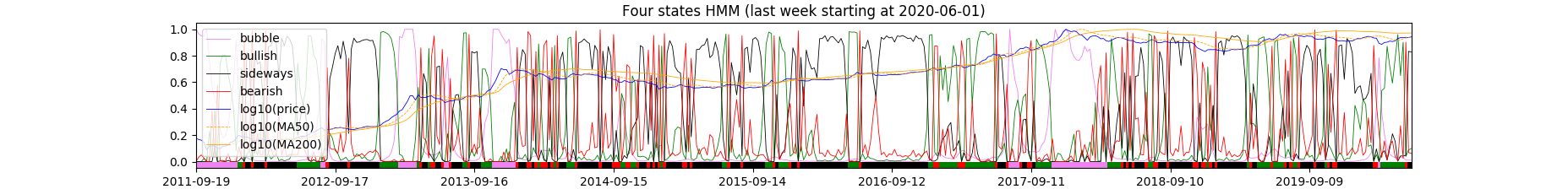 |
|
|
|
|
|
trantute2 (OP)
|
|
August 30, 2020, 08:37:33 PM
Last edit: August 30, 2020, 08:51:03 PM by trantute2 |
|
HMM-Update (siehe unten). Änderungen: - Die Höhe des MA50 und MA200 ist jetzt korrekt(er);
- Die x-Achsenbeschriftung ist jetzt konstant(er);
- Die Halvings sind markiert.
Wie führt man den Code aus: - python3 starten;
- Code reinkopieren.
Oder Code in Datei hmm.py abspeichern und dann aufrufen. HMM bis einschliesslich dieser Woche: 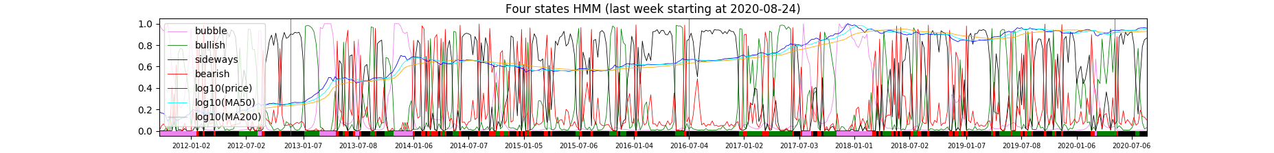 Code: import os;
import re;
import wget; # pip3 install wget
import numpy; # pip3 install numpy
import pandas; # pip3 install pandas
import matplotlib; # pip3 install matplotlib
from hmmlearn import hmm; # pip install --upgrade --user hmmlearn
######################################################################
# weighted mean
def wm(x):
return (x['VOLUME'] * x['PRICE']).sum()/x['VOLUME'].sum();
# weighted mean for rolling window
def rolling_wm(ser):
return (subdata['VOLUME'].loc[ser.index] * subdata['PRICE'].loc[ser.index]).sum()/subdata['VOLUME'].loc[ser.index].sum();
# removes incomplete weeks
def rm(df, column, n):
for i in range(n):
if df[column].iloc[0] != subdata[column].iloc[i]:
return df.iloc[i:df.shape[0]];
return df;
def fill(df, column):
x = numpy.zeros([df.shape[0]]);
c = 0; x[0] = c;
for i in range(df.shape[0]-1):
if df[column].iloc[i] != df[column].iloc[i+1]:
c += 1;
x[i+1] = c;
return x.astype(int);
######################################################################
# download and/or load bitstamp data
file_name = 'bitstampUSD.csv.gz';
# but make sure, that the file is up to date
# if the file already exists locally, the current one
# is not downloaded, thus, remove the local version
if os.path.exists(file_name) == False:
file_name = wget.download('https://api.bitcoincharts.com/v1/csv/bitstampUSD.csv.gz');
data = pandas.read_csv(file_name, compression='gzip', header=None);
data.columns = ['EPOCH', 'PRICE', 'VOLUME'];
data = data.sort_values(by='EPOCH');
data['DATE'] = pandas.to_datetime(data['EPOCH'],unit='s').dt.tz_localize('utc').dt.tz_convert('Europe/Berlin');
data['DAY'] = [str(x) for x in pandas.Series(data['DATE']).dt.date];
# firstly group by day for faster processing
subdata = data.groupby('DAY').first();
subdata['OPEN'] = data.groupby('DAY').first()['PRICE'];
subdata['CLOSE'] = data.groupby('DAY').last()['PRICE'];
subdata['MAX'] = data.groupby('DAY').max()['PRICE'];
subdata['MIN'] = data.groupby('DAY').min()['PRICE'];
subdata['VOLUME'] = data.groupby('DAY').sum()['VOLUME'];
subdata['PRICE'] = data.groupby(['DAY']).apply(wm);
# weighted moving average, not sure whether this makes a difference
rol = subdata['PRICE'].rolling(50); subdata['MA50'] = rol.apply(rolling_wm, raw=False);
rol = subdata['PRICE'].rolling(200); subdata['MA200'] = rol.apply(rolling_wm, raw=False);
#subdata['MA50'] = subdata["PRICE"].rolling(50).mean();
#subdata['MA200'] = subdata["PRICE"].rolling(200).mean();
subdata['RETURN'] = (subdata['CLOSE'] - subdata['OPEN'])/subdata['OPEN'];
subdata['WEEK'] = [str(pandas.Timestamp(x).week) for x in subdata['DATE']];
######################################################################
# not very elegant way to get unique week annotation
# remove first incomplete WEEK
subdata = rm(subdata, 'WEEK', 7);
# remove last incomplete WEEK
subdata = subdata.sort_values(by='EPOCH', ascending=False);
subdata = rm(subdata, 'WEEK', 7);
subdata = subdata.sort_values(by='EPOCH');
subdata['WEEK'] = fill(subdata,'WEEK');
######################################################################
# secondly group by week
subsubdata = subdata.groupby('WEEK').first();
subsubdata['DAY'] = [str(x) for x in pandas.Series(subsubdata['DATE']).dt.date];
subsubdata['OPEN'] = subdata.groupby('WEEK').first()['OPEN'];
subsubdata['CLOSE'] = subdata.groupby('WEEK').last()['CLOSE'];
subsubdata['MAX'] = subdata.groupby('WEEK').max()['MAX'];
subsubdata['MIN'] = subdata.groupby('WEEK').min()['MIN'];
subsubdata['VOLUME'] = subdata.groupby('WEEK').sum()['VOLUME'];
subsubdata['PRICE'] = subdata.groupby(['WEEK']).apply(wm);
subsubdata['LOG10_PRICE'] = numpy.log10(subsubdata['PRICE']);
max_log10_price = numpy.amax(subsubdata['LOG10_PRICE']);
subsubdata['LOG10_PRICE'] = subsubdata['LOG10_PRICE']/max_log10_price;
subsubdata['LOG10_MA50'] = numpy.log10(subsubdata['MA50']);
subsubdata['LOG10_MA50'] = subsubdata['LOG10_MA50']/max_log10_price; # it's all relative to the price
subsubdata['LOG10_MA200'] = numpy.log10(subsubdata['MA200']);
subsubdata['LOG10_MA200'] = subsubdata['LOG10_MA200']/max_log10_price; # it's all relative to the price
subsubdata['RETURN'] = (subsubdata['CLOSE'] - subsubdata['OPEN'])/subsubdata['OPEN'];
# at least not wrong ...
subsubdata = subsubdata.sort_values(by='EPOCH');
# create a model and fit it to data
model = hmm.GaussianHMM(4, "diag", n_iter=1000);
X = numpy.asarray(subsubdata['RETURN']).reshape(-1,1);
fit = model.fit(X);
hidden_states = model.predict(X);
hidden_probs = model.predict_proba(X);
df = pandas.DataFrame(hidden_probs);
df.columns = ['0', '1', '2', '3'];
# my sentiment definition
bubble_state = hidden_states[numpy.where(subsubdata['DATE']=='2011-09-19 15:47:03+0200')[0][0]];
sideways_state = hidden_states[numpy.where(subsubdata['DATE']=='2016-10-03 00:00:18+0200')[0][0]];
bullish_state = hidden_states[numpy.where(subsubdata['DATE']=='2013-02-11 00:57:24+0100')[0][0]];
bearish_state = list(set([0,1,2,3]).difference([bubble_state, sideways_state, bullish_state]))[0];
state_index = {'violet':str(bubble_state), 'green':str(bullish_state), 'black':str(sideways_state), 'red':str(bearish_state)};
state_index_= {str(bubble_state):'violet', str(bullish_state):'green', str(sideways_state):'black', str(bearish_state):'red'};
# plot the result
import matplotlib.pyplot as plt;
fig, ax = plt.subplots(figsize=(2.24,2.24));
df[state_index['violet']].plot(ax=ax, color='violet', linewidth=0.6, label='bubble');
df[state_index['green']].plot(ax=ax, color='green', linewidth=0.6, label='bullish');
df[state_index['black']].plot(ax=ax, color='black', linewidth=0.6, label='sideways');
df[state_index['red']].plot(ax=ax, color='red', linewidth=0.6, label='bearish');
subsubdata['LOG10_PRICE'].plot(ax=ax, color='blue', linewidth=0.6, label='log10(price)');
subsubdata['LOG10_MA50'].plot(ax=ax, color='cyan', linewidth=0.6, label='log10(MA50)');
subsubdata['LOG10_MA200'].plot(ax=ax, color='orange', linewidth=0.6, label='log10(MA200)');
for i in range(len(hidden_states)):
rect = matplotlib.patches.Rectangle((i-0.5,0),1,-0.1,linewidth=1,edgecolor='none',facecolor=state_index_[str(hidden_states[i])]);
ax.add_patch(rect);
blubb = [str(x) for x in subsubdata["DATE"]];
blubb = [re.match('^[0-9]{4}', x).group() for x in blubb];
indices = [];
for i in range(len(blubb)-1):
if blubb[i] != blubb[i+1]:
indices.append(i+1);
quarts = [0, 26];
ticks = [];
for index in indices:
for quart in quarts:
if index + quart > len(blubb):
break;
ticks.append(index + quart);
ticks = numpy.asarray(ticks);
ax.legend();
plt.xticks(ticks=ticks, labels=subsubdata['DAY'].iloc[ticks], rotation='horizontal');
for tick in ax.xaxis.get_major_ticks():
tick.label.set_fontsize(7);
plt.title('Four states HMM (last week starting at ' + subsubdata['DAY'].iloc[subsubdata.shape[0]-1] + ')');
# first halving ~ 1354060800 (2012-11-28)
i = numpy.amax(numpy.where(subsubdata["EPOCH"] < 1354060800));
plt.axvline(i, linewidth=0.6);
# second halving ~ 1468022400 (2016-07-09)
i = numpy.amax(numpy.where(subsubdata["EPOCH"] < 1468022400));
plt.axvline(i, linewidth=0.6);
# third halving ~ 1589155200 (2020-05-11)
i = numpy.amax(numpy.where(subsubdata["EPOCH"] < 1589155200));
plt.axvline(i, linewidth=0.6);
plt.show();
|
|
|
|
|
|
trantute2 (OP)
|
|
August 31, 2020, 08:25:15 PM |
|
Highly fortgeschrittene statistics: 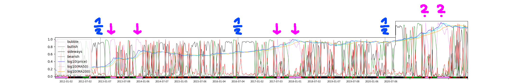 |
|
|
|
|
|